GIS Toolboxes and Plugins

Standard GIS tools provide powerful capabilities for managing, visualising and analyzing spatial data; however, they can sometimes fall short when faced with highly specialized tasks, unique workflows or emerging analytical needs. This limitation arises because built-in tools are designed to cater to general use cases, leaving users seeking solutions for niche or advanced problems. Toolboxes address this challenge by offering a structured set of additional geoprocessing tools, enabling users to perform more complex operations, like spatial statistics, raster modeling or 3D analysis, all within the native environment of the GIS software. For tasks that go beyond even these enhanced functionalities, plugins serve as an invaluable resource. These user-developed add-ons integrate seamlessly into the software, providing specialized features, connections to external data sources, or entirely new analytical frameworks, allowing users to customise their GIS experience to meet specific project demands. Together, toolboxes and plugins expand the horizons of what GIS can achieve, empowering users to tackle diverse and intricate spatial problems effectively.

A toolbox in GIS is a collection of pre-built tools or geoprocessing functions designed to perform specific spatial analysis or data manipulation tasks. It provides a structured way to access built-in capabilities of the GIS software. In QGIS: The "Processing Toolbox" includes tools for vector analysis, raster processing and integration with external libraries like GRASS and SAGA. In ArcGIS: The "ArcToolbox" provides tools for geostatistical analysis, 3D analysis and network analysis.

A plugin in GIS is an add-on or extension that provides additional features, tools or integrations not available in the standard installation of the software. Plugins are often user-developed and community-contributed. Plugins add functionality beyond the built-in capabilities of the GIS software. They require installation, typically through a plugin manager or an online repository. Plugins can be customised or built using programming languages like Python. In ArcGIS: “Spatial Analyst” or “3D Analyst” are plugins (called extensions in ArcGIS) which need to be installed separately. In QGIS: “QuickOSM” plugin is often used to download data from OpenStreetMap or “Layman” plugin can be used to communicate with a Layman data catalogue, connecting desktop GIS and WebGIS.

The Processing Toolbox in QGIS is a centralized interface for accessing a wide array of geoprocessing tools. It acts as a gateway to native QGIS tools, as well as functionalities from integrated external libraries like GRASS GIS, SAGA GIS, GDAL, and Orfeo Toolbox. These tools enable users to perform spatial analysis, data transformation, raster processing, and more.

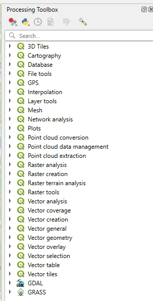
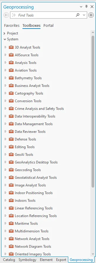
The Processing Toolbox in QGIS and Geoprocessing panel in ArcGIS Pro both provide a set of spatial analysis tools divided into groups by their purpose.

Using the Processing Toolbox in QGIS

1. Accessing the Toolbox:

• Open QGIS.
• Go to Processing > Toolbox to enable it. It appears as a panel on the side of the QGIS interface.

2. Searching for Tools:

• Use the search bar to quickly locate a specific tool by its name (e.g. "Buffer").
• Browse through categories to explore available tools.

3. Workflow for Using Tools:

• Input Selection: Select the input dataset (vector or raster) for the tool. This can be done by browsing through the file system or selecting a layer already loaded in QGIS.
• Parameter Configuration: Set the required parameters for the tool. For example:
  • For a buffer operation: Define the buffer distance and output layer format.
  • For raster calculations: Enter the algebraic expression and specify the output resolution.
• Output Specification: Choose where to save the output (temporary or permanent layer) and define its format (e.g. GeoPackage, Shapefile, TIFF).
• Execution: Click "Run" to execute the tool. Progress is shown in a log window.
• Result Review: The output layer is automatically added to the Layers panel for visualisation and further analysis.

4. Batch Processing:

• Many tools in the Processing Toolbox support batch processing, allowing users to apply the same operation to multiple datasets simultaneously.

5. Model Building:

• The Processing Toolbox integrates with the Model Builder for creating workflows that chain multiple tools together into automated processes.

Exercise: Interpolating Temperature Values Across a Study Area

This exercise demonstrates how to derive meaningful spatial insights from sparse point data, a foundational skill in GIS analysis. Even if you don’t have real-world temperature data, a synthetic dataset with a few points can be created to simulate weather station data.

Problem to Solve: Use weather station data to create a temperature surface for a region. Visualise spatial temperature trends and identify areas of high or low temperature by interpolating temperature values. This is useful for applications such as climate analysis, agriculture planning or environmental monitoring.

Data Needed:

• A set of weather station points (can be a sample dataset or generated synthetically). Each station should have attributes for location (latitude/longitude) and temperature readings (e.g. in °C). Example: CSV file with columns for station name, coordinates and temperature values.

Tools in QGIS Processing Toolbox:

• IDW Interpolation (native QGIS tool) – interpolation algorithm

Workflow

1. Prepare the Data

• Import the weather station point data (e.g, CSV or shapefile) into QGIS.
• Ensure the attribute table contains a column for temperature values.

2. Perform IDW Interpolation

• Open the IDW Interpolation tool from the Processing Toolbox.
• Select the weather station points as the input layer.
• Choose the temperature attribute for interpolation.
• Define the extent and resolution of the output raster based on the study area's boundary.
• Run the tool and save the resulting raster layer (e.g. "Temperature_IDW").

3. Visualize the Results

• Add the raster layer to the QGIS project.
• Apply a colour gradient to the layer.

4. Analyse the Results

• Interpret the temperature trends, such as identifying hotspots or areas with cooler temperatures.

Exercise: Cost Distance Analysis for Optimal Route Planning

Problem to Solve: Identify the least-cost path between two locations based on a cost surface, such as terrain slope or land use. Cost distance analysis is often used in transportation planning, ecological studies (e.g. wildlife corridors) and infrastructure development.

Data Needed:

1. Raster Data:

• Digital Elevation Model (DEM) or land use raster.

2. Vector Data:

• Start and end points (locations) as point layers.

Tools in QGIS Processing Toolbox:

• GDAL Tools:
  • Proximity (Raster Distance): To compute distance rasters.
• Raster Calculator: To create a cost surface.
• Shortest Path (Point to Layer): To calculate the least-cost path.

Workflow

1. Load the Data

• Import the DEM or land use raster and the start/end point vector layers into QGIS.

2. Create a Cost Surface

• If using a DEM: Calculate the slope using the Slope tool from the Processing Toolbox.
• Combine slope and other cost factors (e.g. land use, forested areas) using the Raster Calculator. For example, assign higher costs to steeper slopes or restricted areas:
  "slope_raster" * 2 + "land_use_raster"
• Save the resulting cost surface as a new raster layer.

3. Calculate the Cost Distance

• Use the Proximity (Raster Distance) tool to generate a distance raster from the start point based on the cost surface.

4. Find the Least-Cost Path

• Use the Shortest Path tool with the start and end points, referencing the cost surface raster.
• Save the output as a vector line layer representing the optimal path.

5. Analyse the Results

• Overlay the path with the original cost surface and DEM to visualize the terrain and path efficiency.
• Optionally, calculate path length or cost using the Field Calculator.

Exercise: Analysing Watershed Delineation

Standard tools in QGIS do not support hydrological operations like flow direction, accumulation, and watershed delineation, which require specialized algorithms. Tools from GRASS and SAGA GIS integrate seamlessly into the QGIS Processing Toolbox, enabling users to perform these advanced spatial analyses.

Problem to Solve: Identify areas where water accumulates and delineate watersheds to aid in water resource management.
Data Needed:

• A Digital Elevation Model (DEM) of the study area.
• River or stream network data (optional, for validation).

Tools in QGIS:

GRASS Tools:

• r.watershed: To compute flow direction, accumulation, and watershed boundaries.

SAGA Tools:

• Catchment Area (Flow Accumulation): To calculate flow accumulation.
• Channel Network and Drainage Basins: To generate stream networks.

Workflow:

1. Install SAGA GIS

• Download SAGA GIS binaries
• Install SAGA GIS plugin
• Enable SAGA tools in the “Processing toolbox”

2. Load the Data

• Import the DEM raster into QGIS.
• (Optional) Load vector points to define specific outlets or areas of interest.

3. Preprocessing the DEM

• Use the Fill Sinks (Wang & Liu) tool from the Processing Toolbox to remove depressions and ensure proper flow direction. Save the output as a new DEM.

4. Calculate Flow Direction and Accumulation

• Use the r.watershed tool from GRASS GIS.
• Input the preprocessed DEM and set thresholds for flow accumulation.
• Generate output layers for flow direction, accumulation, and streams.

5. Delineate Watersheds

• Use the Catchment Area (Flow Accumulation) tool or the Channel Network and Drainage Basins tool from SAGA GIS.
• Define watershed boundaries based on the flow direction and accumulation results.

6. Analyze the Results

• Overlay the watershed boundaries with land use or soil data to assess the impact of water flow.
• Visualise stream networks to identify potential sites for water management structures like dams or retention basins.

Expected Outcome:

• A map showing delineated watershed boundaries and stream networks.
• Identification of flow accumulation patterns and key drainage basins.
• Insights into water flow dynamics to inform environmental or engineering decisions.