Introduction to Spatial Analysis

Spatial Analysis in a Nutshell

Spatial analysis is a component of Geographic Information Systems (GIS), which allows users to examine spatial relationships, patterns and trends in geographic data. Analysis generates new data, and that data can be in the form of new layers, tables or simple values. The result of an analysis might express the same variable as the original data (for instance, computing the average value), or a different one (for instance, if we compute a slope layer from an elevation layer).

Spatial analysis can answer questions like:

• "Where should a new warehouse be built to minimize delivery times?"
• "Which agricultural lands fall within flood-prone zones?"
• "How has urban sprawl expanded over the past decade?"
• "What is the shortest route for emergency vehicles to reach an accident site?"

Common spatial analysis techniques include buffering, overlay analysis, spatial interpolation, network analysis and spatial clustering. Each technique serves a specific purpose and is used across various disciplines to solve real-world problems.

For instance, buffering is used to create zones around features, such as a 500-meter buffer around rivers to assess areas at risk of flooding. In urban planning, this technique helps determine the coverage of public facilities, like schools or hospitals, and identify underserved areas. Overlay analysis combines multiple layers of data to derive new insights, such as identifying suitable locations for renewable energy projects by overlaying layers of solar radiation, land use and proximity to infrastructure.

Network analysis focuses on routing and logistics, commonly used in transportation and emergency services. For example, it helps determine the shortest path for ambulances to reach patients or optimize delivery routes for logistics companies. Spatial interpolation is valuable in environmental sciences, where data from weather stations can be interpolated to predict temperature or rainfall across unsampled areas. Similarly, spatial clustering methods like hotspot analysis are applied in public health to identify areas with high concentrations of disease outbreaks, enabling targeted interventions.

By employing these techniques, spatial analysis transforms raw geospatial data into actionable insights, supporting decision-making in fields ranging from environmental management and urban development to public health and disaster response.

Buffer Analysis

A buffer is a zone created around a geographic feature (point, line or polygon) at a specified distance. This zone represents the area of influence or proximity around that feature. Buffer analysis is widely used in GIS for proximity studies and is a foundational spatial analysis tool. Buffer analysis is versatile, forming the foundation for many spatial queries and decision-making processes across fields like environmental science, urban planning, public safety and more.

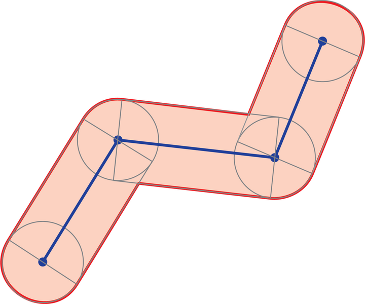
The principle of creating a buffer of a vector feature. Blue is the original (poly)line, gray are the buffers of individual segments and red is the resulting buffer area of the whole line. Source: Bplewe / CC BY-SA 4.0

How It Works:

1. Input Features: Buffers can be created around points (e.g. a school), lines (e.g. a road) or polygons (e.g. a lake).
2. Buffer Distance: A user defines the distance from the feature to determine the extent of the buffer zone. This distance can be uniform (e.g. 1 km buffer for all features) or variable, based on an attribute of the feature (e.g. pollution spread varying with factory size).
3. Buffer Shape: Buffers are typically circular around points, elongated along lines or follow the boundary shape for polygons. Advanced GIS tools also allow creating dissolved buffers, where overlapping buffer zones merge into one, or multi-ring buffers, with multiple zones at increasing distances.
4. Output: The result is a new polygon layer representing the buffer zone(s). This can then be overlaid with other data layers for analysis.

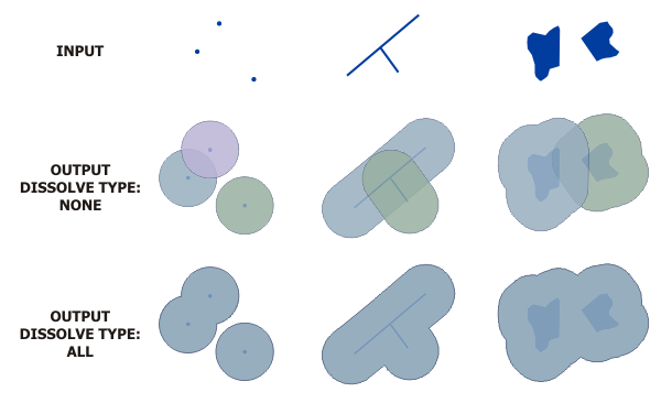
Creating a buffer zone around different types of vector features. From left to right: point features, line features and polygon features. If the resulting buffer zones are dissolved, only one polygon is created in places where the individual buffer zones would overlap (bottom line). Source: ArcGIS Resource Center

Examples of Buffer Analysis:

• Environmental Management:
  • Use Case: Identifying areas at risk of flooding by creating a buffer around rivers.
  • Workflow: A buffer of 500 meters around all rivers is overlaid with land-use data to highlight critical zones like residential areas or farmlands.
• Urban Planning:
  • Use Case: Analyzing public service coverage, such as ensuring schools are within walking distance for communities.
  • Workflow: A 1 km buffer is created around schools and overlaid with population density data to identify underserved neighborhoods.
• Transportation and Safety:
  • Use Case: Evaluating the impact of road construction on nearby habitats.
  • Workflow: Buffers of varying widths are created along proposed road alignments to identify zones where construction might disrupt wildlife or sensitive ecosystems.
• Public Health:
  • Use Case: Assessing the spread of pollutants from industrial facilities.
  • Workflow: A buffer zone (e.g. 2 km) is created around factories, and population data is analysed to identify at-risk communities.
• Emergency Services:
  • Use Case: Optimizing fire station placement to ensure coverage within a specific response time.
  • Workflow: Buffers are drawn around existing fire stations based on their average response radius, highlighting gaps in coverage.

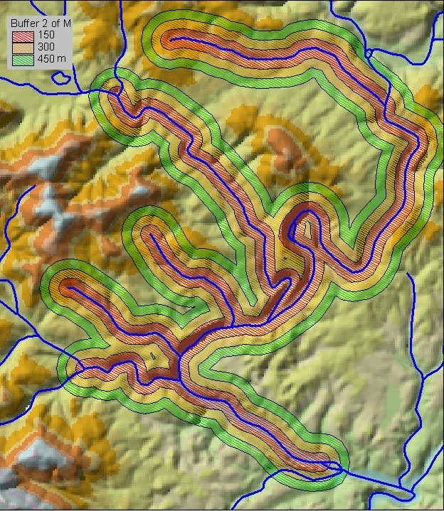
Multi-ring buffer around selected rivers. Rings are created at distances of 150, 300 and 450 metres. The result polygons are dissolved. Source: Ticald622 / CC BY-SA 3.0

Key Considerations:

• Real-World Accuracy: Buffer distance should reflect real-world scenarios, such as the actual spread of pollutants or realistic walking distances.
• Scale and Units: Ensure consistency in map units (meters, kilometers, etc.) to avoid inaccuracies.
• Edge Effects: Buffers near map edges may lead to incomplete zones unless corrected.

Overlay Analysis

Overlay analysis is a fundamental GIS technique used to combine two or more spatial datasets to create a new layer that identifies relationships or patterns between them. By stacking spatial data layers (e.g. land use, elevation and soil types), overlay analysis helps in answering complex spatial questions and supports decision-making across various domains. Overlay analysis can be performed with both vector and raster data. Operations of map algebra are used for raster data.

The process involves:

1. Input Data: Multiple spatial datasets are needed, typically as vector or raster layers.
2. Alignment and Projection: Ensure all layers share the same spatial reference system and alignment.
3. Overlay Operation: Layers are combined through mathematical, logical, or spatial operations to produce a new dataset. The result retains attributes and geometry from the input layers, revealing interactions or overlaps.
4. Analysis: The derived layer is analyzed to extract insights, identify patterns, or make decisions.

Types of vector overlay analysis:

• Union: Combines all input features, retaining all attributes and geometries from both datasets.
  • Example: Analyzing land use and administrative boundaries to evaluate how land use patterns align with jurisdictional areas.
• Intersect: Retains only the overlapping areas between input datasets, combining attributes where they overlap.
  • Example: Identifying regions suitable for agriculture by intersecting layers of fertile soil and areas with sufficient rainfall.
• Erase: Removes the overlapping portion of one dataset from another.
  • Example: Excluding protected areas from a potential development zone layer.
• Clip: Trims one dataset to fit within the boundary of another, maintaining the original data attributes of the clipped features.
  • Example: Extracting city-specific road networks by clipping the road layer to city boundaries.

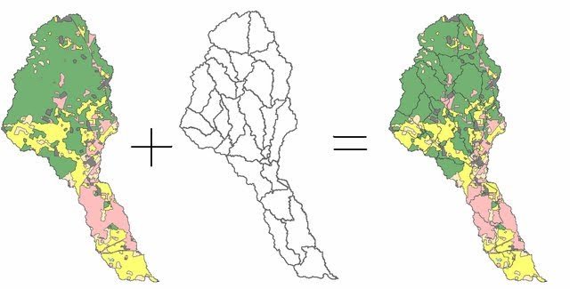
Intersect overlay combines attributes from both input layers in the smallest common regions. Source: Johnson, Nathan & Maidment, David & Katz, Lynn. (2005). ArcGIS and HSPF model development.

Types of raster overlay analysis:

• Combines cell values from multiple raster layers using mathematical or logical operations (e.g. addition, subtraction, or Boolean logic).
  • Example: Adding rainfall and elevation layers to identify areas prone to landslides.
• Weighted overlay is a common raster analysis where layers are assigned weights based on their importance to the analysis goal.
  • Example: Prioritizing conservation areas by combining layers of biodiversity, proximity to water, and human impact, each weighted by its significance.

Examples of Overlay Analysis:

• Environmental Management: Identifying flood-prone areas by overlaying layers of elevation, proximity to rivers, and rainfall intensity. This helps in disaster preparedness and land-use planning.
• Urban Planning: Selecting the best location for a new park by overlaying population density, land availability, and proximity to existing green spaces.
• Public Health: Mapping areas at high risk for mosquito-borne diseases by overlaying layers of stagnant water locations, population density, and temperature suitability for mosquito breeding.
• Infrastructure Development: Planning a highway by overlaying layers of land ownership, soil type, and protected environmental areas to minimize conflicts and impacts.
• Wildlife Conservation: Determining critical habitats for conservation by overlaying species distribution, vegetation type, and human activity layers.

Buffer and Overlay Analysis Exercise: Noise Pollution Analysis

Problem to Solve: Assess noise pollution impact zones around major roads or highways to guide urban planning.
Data Needed:

• Vector data: Road network (polylines).
• Vector data: Population density or residential areas (polygons).

Tools in QGIS:

• Buffer: Create noise impact zones around the roads.
• Intersection or Spatial Join: Identify residential areas within the noise zones.

Workflow:

1. Load the road network data into QGIS.
2. Use the Buffer tool to generate buffer zones around roads (e.g. 100 meters for high traffic roads).
3. Overlay the buffer with residential area polygons using the Intersection tool.
4. Visually analyse the output to estimate the population affected by noise pollution.