Key Concepts

Radiometric classes: Image pixel classification deals with samples (or pixels) to be classified. It is assumed that there exists a finite set of possible radiometric classes (class labels)

Ω = {ω1, ω2,…, ωk,…, ωK}

The elements of ωk of Ω are called radiometric classes, and Ω is the set of radiometric classes. The number of classes to be distinguished is

K = card (Ω) = number of classes

The K classes ωk are represented by a distinct name or class label, defined by the community of GIS users.

The example of agricultural crop classification in a satellite image of a farming area in the Flevopolder, the Netherlands, illustrates the idea of a set of classes. The image is recorded by the Thematic Mapper sensor of the Landsat satellite, which measures reflected sunlight in six spectral bands (visible and infrared) with a spatial resolution of 30 m (Figure 5). Let Ω be the seven dominant crops defining the classes of the classification, i.e.

Ω = {Grass, Wheat, Potatoes, Sugar-beets, Beans, Peas, and Onions}

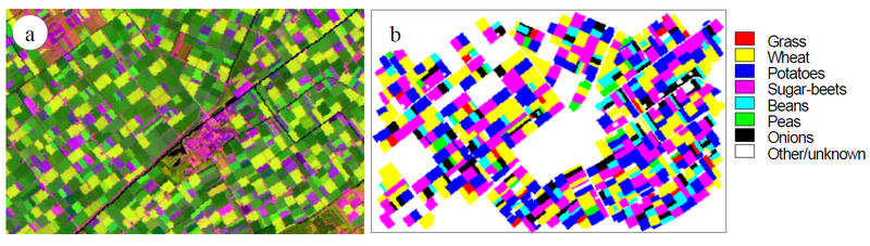
Figure 5. Detection and classification of agricultural fields in RS images. (a) The Flevopolder Landsat-TM images, obtained on July 7, 1987, of the Biddinghuizen area, in Bands 5, 4, and 3 (RGB). (b) Land cover map of 1987, showing seven dominant crops.

The image classification task is then the task of classifying and recognising crops in the area. This specific definition of Ω excludes every other class; a village, a few canals, some forested areas, roads, and farmhouses, although present in the area, are not included in the classification results. Together, these constitute the unknown class ω0.

The set Ω of classes may be defined quite differently depending on the application. The definition of Ω is predominantly a question of application.

Thematic maps: Image classification is the process used to produce 'thematic maps' from imagery. The themes can range, for example, from categories or object classes such as soil, vegetation, and surface water (also referred to as the Radiometric class above). Therefore, to produce a thematic map, the class 'Labels' at each pixel replaces photon counts.

Similarity between pixels, or groups of pixels: In classification, for example, we want to label areas on the ground that have similar physical characteristics. We do this by grouping data with similar characteristics.

Parametric or Nonparametric Classification: Classification algorithms can be categorised into two types: parametric and nonparametric. Parametric algorithms assume a particular statistical distribution of class, commonly the normal distribution, and require estimates of the distribution parameters from the training sample, such as the mean vector and covariance matrix, for classification. Nonparametric algorithms make no assumptions about the probability distribution and are often considered robust because they may work well for a wide variety of class distributions; however, they require a considerable number of training samples.

Formation of Clusters: The core idea is that pixels originating from spectrally similar areas or land cover types (classes) form compact clusters or groups. These groupings are known as "clusters" and are defined as adjacent points in the feature space. For example, feature vectors of water areas typically form a compact cluster, as do those for grass or trees.

Training for defining these distinct clusters: Typically, distinct clusters that correspond to different radiometric classes are identified in the feature space through a "training" process. Each feature vector from a multi-band image can be plotted within this space. This principle enables a comparison of each pixel against these predefined clusters, allowing for assignment to the class that fits best.

The definition of the clusters is an interactive process and is carried out during the training process. Comparison of individual pixels with clusters is performed using classifier algorithms.

Training involves selecting pixels to train the classifier to recognise the desired classes, and classification involves determining decision boundaries that partition the feature space according to the properties of the training pixels. This step is either supervised by the analyst or unsupervised with the aid of a computer algorithm.

In principle, the training sample is a collection of [d, ω] representative of the application, i.e. measurement vectors of known identity, which are assumed to be representative of the classes of interest. Adequate training samples must be available to estimate the parameters of the probability distribution.

Training samples are collected using regions of interest (ROI). ROI are selected on:

• Define the number of classes.
• Class-homogeneous sites, without mixtures among classes.
• Representation of full within-class variability.
• Often, more than one site or area is needed per class.
• Some classes may have a small spatial extent, e.g., an 'asphalt' road.
• Analyse training samples before classification.

A multi-dimensional graph where measurement vectors d are plotted. Each pixel corresponds to one point in feature space. Clusters of points in feature space correspond to distinct object classes.

Figure 6 illustrates a 2D feature space where clusters of five specific land cover types (classes), such as Water and Trees, are plotted.

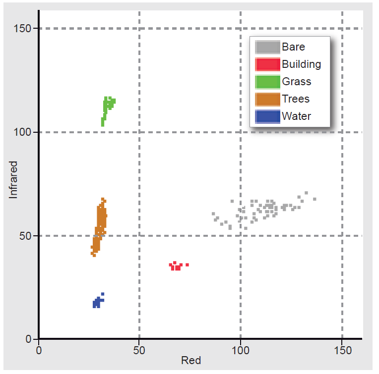
Figure 6. A 2D feature space showing the respective clusters of five classes; note that each class occupies a limited area in the feature space.

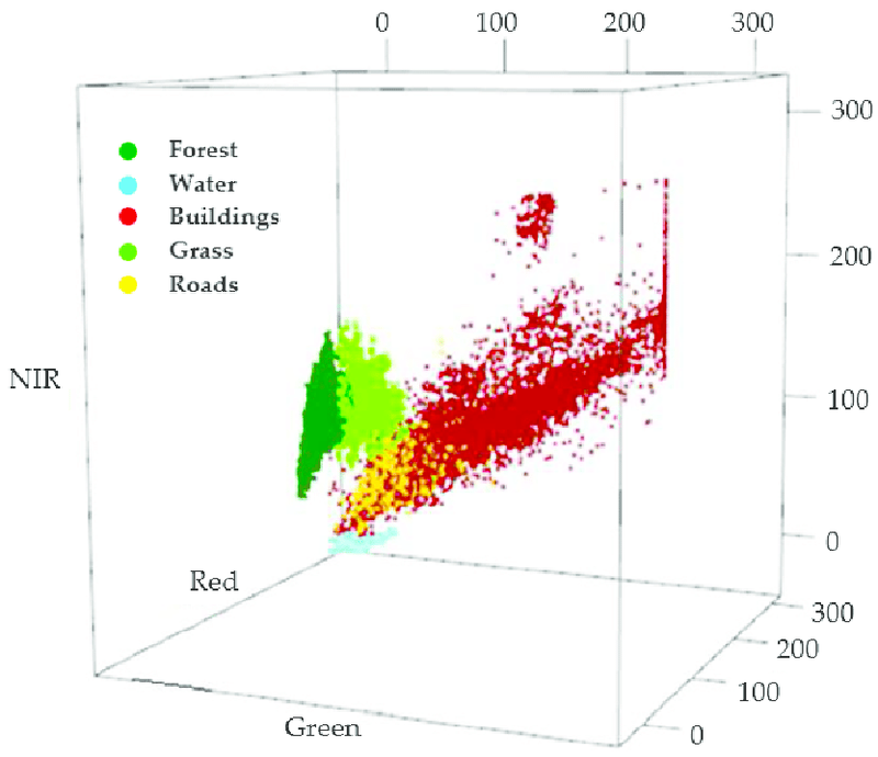
Figure 7. illustrates a 3D feature space where the training pixels for five land cover classes in the Green, Red, and NIR are plotted.

Level-Slice Classifier: This classifier, also known as a box or parallelepiped classifier, is the simplest classification method. A set of K-dimensional boxes, centred at the estimated class mean vectors, are placed in N-dimensional feature space (N is the number of spectral bands). If an unlabeled pixel vector lies within one of the boxes, it is assigned that class label. Specification of the box limits is typically in terms of the data extent in each dimension, for example, ±1 standard deviation about the mean in each band. The delineation of the boxes can also be done directly by the analyst in feature space in an interactive manner. Since the boxes are aligned with the data axes, classification labelling of the whole image can be achieved quickly with hardware or software look-up tables (LUTs), and the resulting map can be viewed simultaneously while manipulating the feature space boxes. A complication occurs if a pixel vector falls within two or more boxes (the boxes can overlap unless that is explicitly prohibited). A decision on a pixel’s label must then be made with another algorithm, such as the nearest mean.

By its nature, the level-slice algorithm also creates an “unlabeled” class referred to as the Unclassified pixels, consisting of all pixel vectors that do not fall within any of the designated boxes.

Hard versus Soft Classification: Labelling of pixels accomplished by partitioning the feature space.

• Hard classification results in one class per pixel.
• Soft classification results in multiple classes per pixel, each with an associated likelihood.
• Soft classification is more accurate and descriptive of reality, accommodating within- and between-class variation, as well as class mixing.

Density slicing: classification using a single band. In theory, it is possible to base a classification on a single spectral band, using single-band classification. DS is a technique whereby the photon counts distributed along the horizontal axis of an image histogram are divided into a series of user-specified intervals or slices. The number of slices and the boundaries between the slices depend on the different object classes in the study area.

Multi-spectral classification: classification using many bands.