Remote Sensing Image Classification

Reading time
Content
Remote sensing involves capturing data about the object surface using sensors, which is then processed to extract meaningful information, often in the form of maps or thematic classifications. Image classification is a core technique in this process, transforming raw image data into object classes or thematic maps, such as land cover maps. Classified images serve as input for Geographic Information Systems (GIS), supporting various analyses and decision-making processes. For example, the European Commission mandates that national governments verify crop subsidy claims, which involves initial inventories using image classification, followed by field checks.
The application problem in this course is to identify scene objects, such as pistachio crop fields and roads, classify them, and estimate their parameters.
Remote sensing image classification is a process used to extract information from remotely sensed images by assigning pixels to specific object class labels or thematic classes based on their characteristics. It is one of the techniques within the domain of machine learning that allows a computer to perform an interpretation according to defined conditions. This process transforms remote sensing images into land cover types (classes), such as soil type or crop disease maps, including those related to pistachio trees.
The basic assumption for image classification is that a specific part of the feature space corresponds to a specific class, meaning spectrally similar pixels group together to form compact clusters.
Image Space
In remote sensing, radiometric measurements are primarily the outputs of a sensor. For this purpose, the sensor may be an RGB camera or a satellite-borne multi-spectral scanner, such as Sentinel-2.
A digital image is a 2-dimensional matrix in which a typical element is referred to by (xi, yj) where i=1, 2 ..., r and j=1,2 ..., c (with r: number of rows, c: number of columns). At each element in the image, a set of photon counts is available in several spectral bands (referred to as ‘Image Space’ – Figure 2).
Let d(xi, yj) denote samples corresponding to the N-dimensional measurement space D at image sample position (xi, yj), where N is the number of spectral bands. The sensor's output is a set of N measurements, each corresponding to a single channel of the scanner. The set of all measurements referring to the same sample is combined in the measurement vector
d = [d1 d2 … dN]T
where T is the matrix transpose operator. Hereafter, the measurement vector d(xi, yj) is abbreviated to d. The vectors are denoted in boldface type (for instance, d or p).
The dimension N of d determines the number of bands that are used for classification.
N = dim(d) = number of measurements (or bands)
The measurement vector d points to a single point in the N-dimensional measurement space D. Measurements are represented as numerical data with a physical dimension of photon counts.
In conclusion, d is the collection of remotely sensed multispectral data at a fixed time.
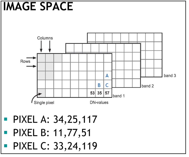
Figure 2. An image file comprises a digital image for each of the sensor's spectral bands. For every band, the photon counts or DN-values are stored in a row-column arrangement. N = 3 (number of bands).
Feature Space
When considering a two-band image, we can say that the two DNs for a ‘surface element’ or the GRC of the sensor are components of a 2D vector [d1, d2], which forms the feature vector (Figure 3). An example of a feature vector is [13, 55], which indicates that the conjugate pixels of band-1 and band-2 have DNs 13 and 55. This vector can be plotted in a two-dimensional graph.
Similarly, we can visualise a 3D feature vector [d1, d2, d3] of a cell in a three-band image found in a three-dimensional graph. A graph that shows the feature vectors is called a feature space, or feature space plot or scatter plot. Figure 3 illustrates how a feature vector (related to one GRC) is plotted in the feature space for two and three bands. Two-dimensional feature-space plots are the most common.
Note that plotting the values is difficult for a four- or more-dimensional case, even though the concept remains the same. A practical solution when dealing with four or more bands is to plot all possible combinations of two bands separately. For four bands, this already yields six combinations: bands-1 and 2, 1 and 3, 1 and 4, bands-2 and 3, 2 and 4, and bands-3 and 4.
Plotting all the feature vectors of an image pair yields a 2D scatter plot of many scatter plot points (Figure 4). A 2D scatterplot provides information about pixel value pairs that occur within a two-band image. Note that some combinations will occur more frequently.
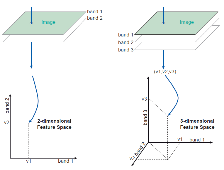
Figure 3. Plotting of the pixel values of a GRC in the feature space for a two-band and three-band image.
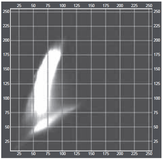
Figure 4. Scatterplot of two bands of an RS image. Note the units along the x- and y-axes. The intensity at a point in the feature space is related to the number of cells at that point.
Spectral Features
Image classification aims to assign pixels to specific object classes based on their spectral features (i.e., their feature vectors) by comparing them to predefined clusters in feature space.
Mapping to RGB Channels for Display: Computer image displays typically convert image data into a continuous, analog image using red, green, and blue (RGB) primary screen colours. To achieve this, three bands of a multispectral image are processed by hardware Look-Up Tables (LUTs) that convert photon counts (their integer DNs) into the Red, Green, and Blue display channels. With a 24-bit display system, each band is assigned to one of three 8-bit integers corresponding to the display colours (R, G, B). However, RGB is not perceptually uniform — similar numerical differences don’t necessarily mean similar visual differences.
When considering an image with three RGB spectral bands, these three bands form a three-dimensional feature vector. This vector can be visualised and plotted in a three-dimensional graph, which is referred to as a feature space or a scatter plot. This concept is directly analogous to an "RGB cube space."
Cube Spaces
Images are often represented in the RGB colour space (Red, Green, Blue). Each pixel has three values.
The RGB colour cube is a conceptual representation of the RGB (Red, Green, Blue) data. It functions as a dataspace for images that are captured by 3-band sensors, such as RGB cameras. Here's a breakdown of what the colour cube entails:
The RGB cube space is a three-dimensional feature space specifically designed for visualising and processing three-band remote sensing data, where each axis represents the scaled photon counts of the Red, Green, or Blue bands.
Dimensions and Data Cells When RGB data is scaled to a byte range (0 to 255), the colour cube can be thought of as containing 256^3, or 2^24, data cells or 3-dimensional bins.
This "colour cube" visually represents all possible combinations of these Red, Green, and Blue photon count values. The axes of this 3D space correspond to the intensity of the red, green, and blue components. For an 8-bit per channel system, this cube ranges from (Red=0, Green=0, Blue=0) (black) to (Red=255, Green=255, Blue=255). Black (RGB = 0) represents a common point at the origin of this cube, and the maximum values (e.g., 255 for each channel) represent saturation levels determined by scaling the photon counts. This "colour cube" is a specific type of feature space for three-band data, allowing the visualisation of spectral information in three dimensions, similar to how a two-band image can be plotted in a 2D scatter plot.
The fundamental principle underlying the use of such a space for image classification is that different materials (or land cover types) exhibit distinct spectral characteristics. Consequently, spectrally similar pixels tend to group, forming compact clusters within this multi-dimensional feature space, including the RGB cube space.
Mapping to Other Colour Spaces:
To improve segmentation and clustering performance, images are often converted from RGB to alternative colour spaces (Table 1).
The content and surface of the RGB colour cube can be mapped into other coordinate systems. For instance, it can be separated into:
Intensity (I): This is a multiplicative factor, typically the sum of the Red, Green, and Blue photon counts (scaled to a numerical range), such as (Red+Green+Blue)/3. Illumination conditions, such as shadows and shading, can influence this "intensity" factor.
Orthogonal Colour Features (m1, m2): These are two orthogonal axes that define a colour triangle within the sum-normalised colour space. This m1m2I transform is preferred over systems like HSV (Hue, Saturation, Value) for quantitative analysis because m1 and m2 are mathematically independent and do not suffer from noise amplification at low saturation, unlike hue. The concept of using orthogonal axes is generalizable to any number of spectral bands.
Purpose in Analysis: The transformation of raw RGB data (which can be correlated and redundant) from the colour cube into features like m1, m2, and I is a form of feature extraction. The goal is to separate possible information from redundant data and provide a more stable and robust representation of an object's relative reflectance characteristics, which is crucial for tasks like object classification.
Table 1. To improve segmentation and clustering performance, images are often converted from RGB to alternative colour spaces:
| Colour Space | Components | Why Use it in Segmentation |
|---|---|---|
| I | Intensity (I) | This is a multiplicative factor, typically the sum of the Red, Green, and Blue photon counts (scaled to a numerical range), such as (Red+Green+Blue)/3. |
| HSV | Hue, Saturation, Value | Separates colour from intensity; Hue is great for identifying colours regardless of lighting. |
| m1m2I | Orthogonal Colour Features (m1, m2), and Intensity (I) | The m1m2 features are a pair of orthogonal colour features that, together with Intensity (I), form an alternative coordinate system for representing RGB (Red, Green, Blue) data. |
| Normalized RGB | r = R/(R+G+B), etc. | A small constant (e.g., 0.001) is often added to the denominator to prevent division by zero. |