The Classification Process

Reading time
Content
The process of image classification typically involves five steps (Figure 8):
- Selection and Preparation of RS Images: Choosing appropriate sensor, acquisition date(s), and wavelength bands based on the classification goal. This includes consideration of band correlation, where similar spectral reflection in two bands can lead to redundant information and disturb the classification.
- Definition of Clusters in Feature Space: This can be done via supervised or unsupervised methods. In supervised classification, the operator defines the clusters during the training process. In contrast, unsupervised classification involves a clustering algorithm that automatically identifies and determines the number of clusters in the feature space.
- Selection of the Classification Algorithm: Once the spectral classes have been defined in the feature space, the operator needs to decide on how the pixels (based on their feature vectors) are to be assigned to the classes. The assignment can be based on different criteria.
- Running the Actual Classification: Once the training data have been established and the classifier algorithm selected, the actual classification can be carried out. This means that, based on its DNs, each “multi-band pixel” in the image is assigned to one of the predefined classes (Figure 9).
- Validation of the Result: Once the classified image has been produced, its quality is assessed by comparing it to reference data (ground truth). This requires the selection of a sampling technique, the generation of an error matrix, and the calculation of error parameters
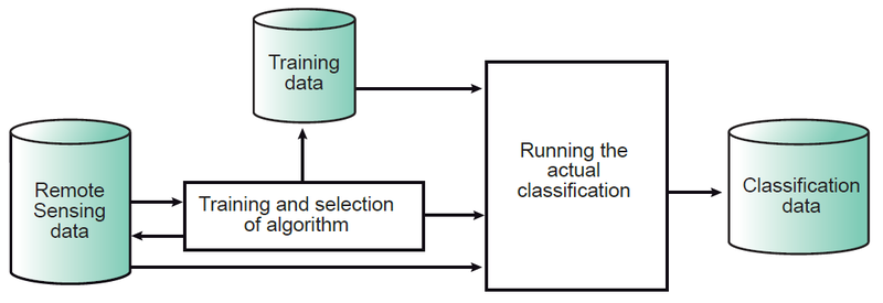
Figure 8. The classification process; the most important component is the training, in combination with the selection of the algorithm.
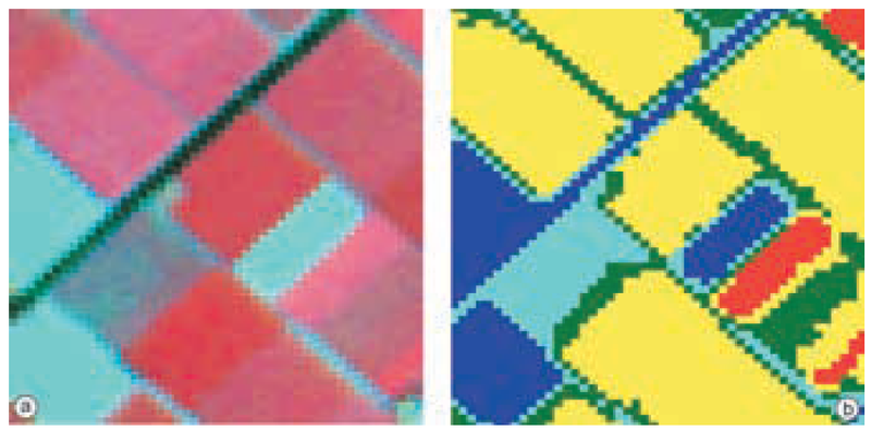
Figure 9. The result of the classification of a multi-band image (a) is an image in which each pixel is assigned to some thematic class (b).
Supervised Classification: An operator defines the spectral characteristics of classes by identifying "sample areas (training areas)". This requires the operator to be "familiar with the area of interest" and know where to find the classes, often through field observations. The principle is that a pixel is assigned to a class by comparing its feature vector to these predefined clusters in feature space. Training samples are collected using "regions of interest (ROI)" which are selected in homogeneous areas.
In supervised classification, the statistical data of classes play a pivotal role in characterising clusters within the feature space, which is the foundation upon which image classification operates. The statistical data (such as means and covariance matrices) are estimated from training samples. These training samples should be representative of the class and cover its within-class variability.
The clusters should not, or only partially, overlap with one another; otherwise, a reliable separation is not possible. For a specific data set, some classes may have significant spectral overlap, which, in principle, means that these classes cannot be discriminated by image classification. Solutions include adding other spectral bands and/or images acquired at different times (Figure 10).
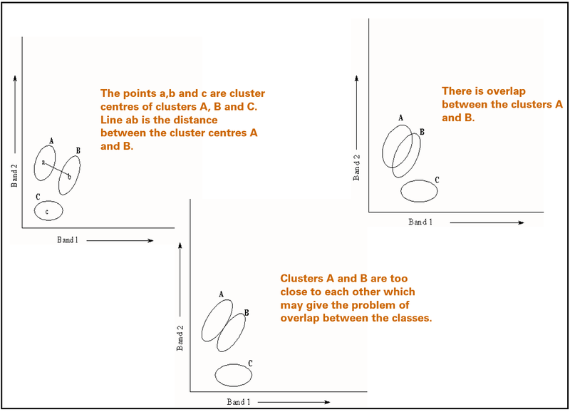
Figure 10. Visualising Clusters and Overlap. Shows the spectral overlaps of the clusters in the feature space for supervised classification. Spectral overlap occurs when these clusters, representing different classes, are not distinctly separated in the feature space. This means that some pixel value combinations for one class might fall into the region predominantly occupied by another class, making their differentiation challenging.
In the supervised classification, the derived cluster statistics are then used to classify the complete image using a selected classification algorithm.
Unsupervised Classification is used when knowledge of the area is insufficient or classes are undefined. Clustering algorithms automatically "partition the feature space into several clusters" based on spectral similarities. A common approach involves the user defining the maximum number of clusters; the computer then locates arbitrary mean vectors as cluster centres, assigns pixels to the nearest centre, and recalculates centres iteratively until they stabilise. Clusters with too few points can be eliminated or merged.
Figure 11 illustrates the results of a clustering algorithm applied to a dataset. Note that the cluster centres coincide with the high-density areas in the feature space.
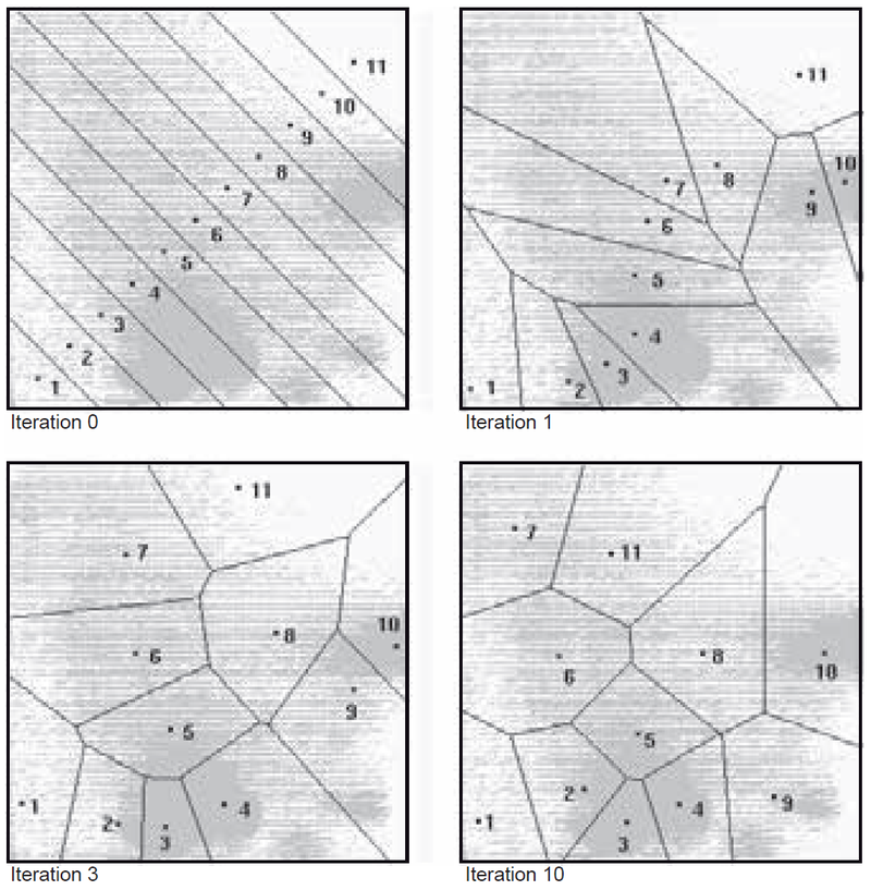
Figure 11. The subsequent results of an iterative clustering algorithm on a sample dataset.
Classification Algorithms:
After the training sample sets have been defined, classification of the image can be carried out by applying a classification algorithm. Several classification algorithms exist. The choice of the algorithm depends on the purpose of the classification and the characteristics of the image and training data. The operator needs to decide if a reject or unknown class is allowed. In the following, three classifier algorithms are described.
First the box classifier is explained—its simplicity helps in understanding the principle. In practice, the box classifier is hardly ever used, however; minimum distance to mean and the maximum likelihood classifiers are most frequently used.
Box Classifier (Level-Slice/Parallelepiped): Simplest, defines upper and lower limits for each band and class, creating box-like areas in feature space. Pixels falling within a box are assigned its label. Can result in "unknown" or "reject" classes, and overlap can cause arbitrary assignment. The number of boxes depends on the number of classes. During classification, every feature vector of an input (two-band) image will be checked to see if it falls in any of the boxes. If so, the cell will get the class label of the box it belongs to. Cells that do not fall inside any of the boxes will be assigned the “unknown class”, sometimes also referred to as the “reject class” (Figure 12).
The disadvantage of the box classifier is the overlap between classes. In such a case, a cell is arbitrarily assigned the label of the first box it encounters.
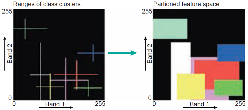
Figure 12. Principle of the box classification in a case of two-dimensional feature space partitioning.
Minimum Distance to Mean (MDM): Assigns a pixel to the class whose cluster centre (mean) is closest. Does not account for class variability. A threshold distance can be set to prevent the assignment of distant points.
Figure 6.14 illustrates how a feature space is partitioned based on the cluster centres. One of the disadvantages of the MDM classifier is that points that are at a large distance from a cluster centre may still be assigned to this centre.
This problem can be overcome by defining a threshold value that limits the search distance. Figure 13 illustrates the effect; the threshold distance to the centre is shown as a circle.
A further disadvantage of the MDM classifier is that it does not account for class variability: some clusters are small and dense, while others are large and dispersed. Maximum likelihood classification, however, does take class variability into account.
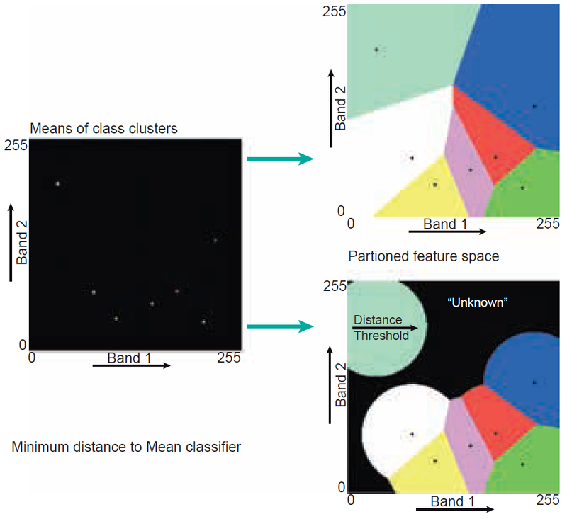
Figure 13. Principle of the minimum distance to mean classification in a two-dimensional situation. The decision boundaries are shown for a situation without threshold distance (upper right) and one with threshold distance (lower right).
Maximum Likelihood (ML): Most frequently used, considers not only cluster centres but also shape, size, and orientation of clusters using probability. Assigns pixel to class with the highest probability. Most ML classifiers assume that the statistics of the clusters follow a normal (Gaussian) distribution.
Maximum likelihood also allows the operator to define a threshold distance by specifying a maximum probability value. A small ellipse centred on the mean describes the values with the highest probability of membership of a class. Progressively larger ellipses surrounding the centre represent contours of probability of membership to a class, with the likelihood decreasing the further away from the centre. Figure 14 illustrates the decision boundaries for a scenario with and without a threshold distance.
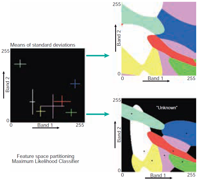
Figure 14. Principle of maximum likelihood classification. The decision boundaries are shown for a situation without threshold distance (upper right) and one with threshold distance (lower right).
Iterative Optimisation (Migrating Means/ISODATA): Estimates initial cluster centres, assigns pixels to nearest centre, recalculates means, and repeats until centres stabilise. The user specifies the number of clusters. Allows for merging and splitting of clusters based on criteria like minimum points or elongated shapes.
Validation of the classification results
Purpose: To check the actual quality and reliability of the classification result.
Methodology: Comparing classified output to "true class" data (ground truth or higher accuracy sources like aerial photos).
Sampling Schemes: Strategies for selecting pixels to test, including simple random sampling and stratified random sampling. Choices involve design, number of samples (determined by sampling theory), and sample unit area.
Error Matrix (Confusion/Contingency Matrix): A comparison is made by creating an error matrix from which various accuracy measures can be calculated. The actual class is preferably derived from field observations. Sometimes, sources with higher accuracy, such as drone images, are used as a reference.
Error matrix is a table comparing classified classes to reference classes.
Once sampling for validation has been carried out and the data collected, an error matrix, also sometimes called a confusion matrix or a contingency matrix, can be established (Table 6.2). In the table, four classes (A, B, C, D) are listed. A total of 163 samples were collected. The table shows that, for example, 53 cases of A were found in the real world (‘reference’), while the classification result yielded 61 cases of a; in 35 cases, they agree.
The first and most commonly cited measure of mapping accuracy is the overall accuracy, or proportion correctly classified (PCC). Overall accuracy is the number of correctly classified pixels (i.e. the sum of the diagonal cells in the error matrix) divided by the total number of pixels checked. In Table 2, the overall accuracy is (35 + 11 + 38 + 2)=163 = 53%. The overall accuracy yields one value for the result as a whole.
- Overall Accuracy: Total correctly classified samples divided by total samples.
- Error of Omission (Type II Error): Samples from a reference class that were incorrectly omitted from that class in the classification (misclassified as another class). Calculated per column. Corresponds to Producer Accuracy.
- Error of Commission (Type I Error): Samples classified into a particular class that belong to a different reference class. Calculated per row. Corresponds to User Accuracy.
- User Accuracy: Probability that a pixel labelled as a particular class belongs to that class.
- Producer Accuracy: Probability that a reference class is correctly mapped as that class.
Table 2. The error matrix with derived errors and accuracy expressed as percentages. A, B, C and D refer to the reference classes; a, b, c and d refer to the classes in the classification result. Overall accuracy is 53 %.
| A | B | C | D | Total | Error of Ommission (%) | User Accuracy (%) | |
|---|---|---|---|---|---|---|---|
| a | 35 | 14 | 11 | 1 | 61 | 43 | 57 |
| b | 4 | 11 | 3 | 0 | 18 | 39 | 61 |
| c | 12 | 9 | 38 | 4 | 63 | 40 | 60 |
| d | 2 | 5 | 12 | 2 | 21 | 90 | 10 |
| Total | 53 | 39 | 64 | 7 | 163 | ||
| Error of Ommission | 34 | 72 | 41 | 71 | |||
| Producer Accuracy | 66 | 28 | 59 | 29 |